Application
The PyBioMed Python package can generate various feature vectors for molecular structure, protein sequences and DNA sequences. The PyBioMed package would be applied to solve many tasks in the field of cheminformatics, bioinformatics and systems biology. We will introduce five examples of its applications including Caco-2 cell permeability, aqueous solubility, drug–target interaction data, protein subcellular location, and nucleosome positioning in genomes. All datasets and Python scripts used in the next five examples can be download on https://github.com/gadsbyfly/PyBioMed/tree/master/PyBioMed/example.
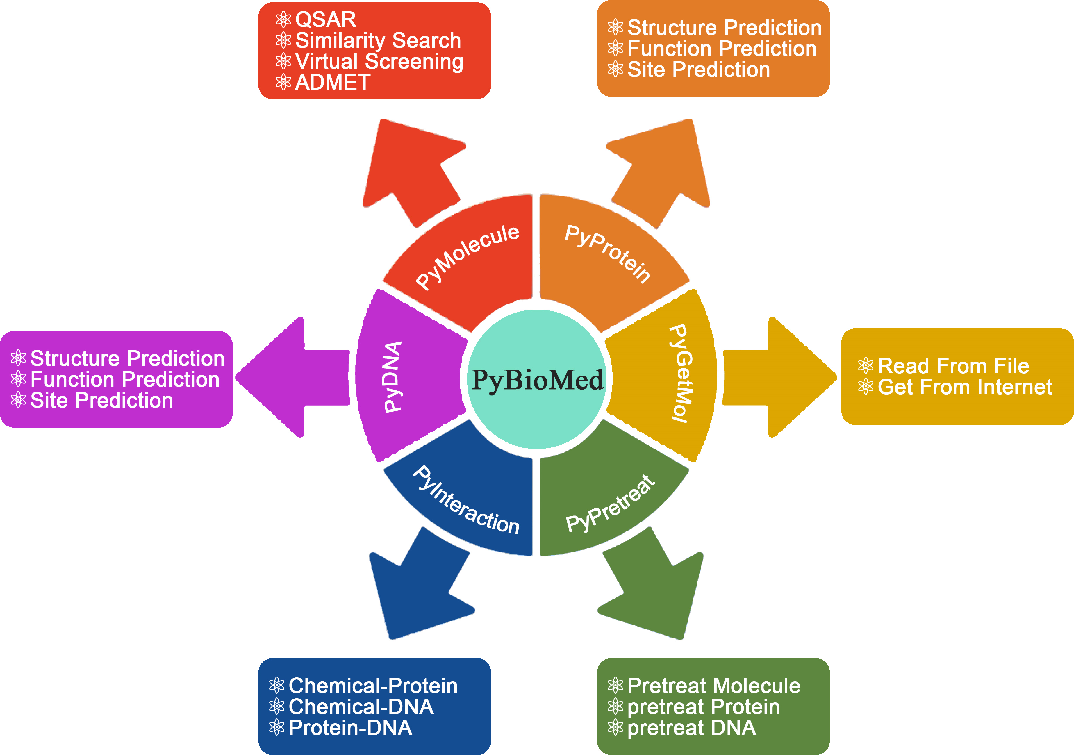
The overview of PyBioMed python package. PyBioMed could calculate various molecular descriptors from chemicals, proteins, DNAs/RNAs and their interactions. PyBioMed can also pretreat molecules, protein sequences and DNA sequences.
Application 1 Prediction of Caco-2 Cell Permeability
Caco-2 cell monolayer model is a popular surrogate in predicting the in vitro human intestinal permeability of a drug due to its morphological and functional similarity with human enterocytes. Oral administration of drugs is the preferred route and a major goal in the development of new drugs because of its ease and patient compliance. Before an oral drug reaches the systemic circulation, it must pass through intestinal cell membranes via passive diffusion, carrier-mediated uptake or active transport processes. Bioavailability, reflecting the drug proportion in the circulatory system, is a significant index of drug efficacy. Screening for absorption ability is one of the most important parts of assessing oral bioavailability. Caco-2 cell line is a popular surrogate for the human intestinal epithelium to estimate in vivo drug permeability due to their morphological and functional similarities with human enterocytes. To build a Caco-2 cell permeability prediction model, we use the PyBioMed package to calculate molecular features and then the Random Forest (RF) method was applied to build Caco-2 cell permeability classification model. The benchmark data set for building the Caco-2 cell permeability predictor was taken from (NN Wang et al. 2016). The dataset contains 1272 compounds.

The receiver operating characteristic curve of Caco-2 classification.
1 2 3 4 5 6 7 8 9 10 11 12 13 14 15 16 17 18 19 20 21 22 23 24 25 26 27 28 29 30 31 32 33 34 35 36 37 38 39 40 41 42 43 44 45 46 47 48 49 50 51 52 53 54 55 56 57 58 59 | from PyBioMed import Pymolecule
import pandas as pd
from sklearn.ensemble import RandomForestClassifier
from sklearn import metrics
from matplotlib import pyplot as plt
#==============================================================================
# load the data
#==============================================================================
train_set = pd.read_excel('./example/caco2/caco2.xlsx',sheetname=0) #change the path to your own path
test_set = pd.read_excel('./example/caco2/caco2.xlsx',sheetname=1) #change the path to your own path
train_set_smi = train_set['smi']
test_set_smi = test_set['smi']
train_set_label = train_set[['label']]
test_set_label = test_set[['label']]
#==============================================================================
# calculating molecular descriptors to a descriptors dataframe
#==============================================================================
def calculate_des(smi):
des = {}
drugclass=Pymolecule.PyMolecule()
drugclass.ReadMolFromSmile(smi)
des.update(drugclass.GetMoran())
des.update(drugclass.GetMOE())
return pd.DataFrame({smi:(des)}).T
train_set_des = pd.concat(map(calculate_des,list(train_set_smi)))
test_set_des = pd.concat(map(calculate_des,list(test_set_smi)))
#==============================================================================
# building the model and predicting the test set
#==============================================================================
clf = RandomForestClassifier(n_estimators=500,max_features='sqrt', n_jobs=-1, max_depth=None,random_state=0)
clf.fit(train_set_des,train_set_label)
proba = clf.predict_proba(test_set_des)[:,1]
predict_label = clf.predict(test_set_des)
#==============================================================================
# Calculating auc score
#==============================================================================
AUC_score = round(metrics.roc_auc_score(test_set_label, proba),2)
TPR = round(metrics.recall_score(test_set_label, predict_label),2)
ACC = round(metrics.accuracy_score(test_set_label, predict_label),2)
P = float(test_set_label.sum())
N = test_set_label.shape[0] - P
SPE = round((P/N+1.0)*ACC-TPR*P/N,2)
matthews_corrcoef = round(metrics.matthews_corrcoef(test_set_label, predict_label),2)
f1_score = round(metrics.f1_score(test_set_label, predict_label), 2)
fpr_cv, tpr_cv, thresholds_cv = metrics.roc_curve(test_set_label, proba)
#==============================================================================
# plotting the auc plot
#==============================================================================
plt.figure(figsize = (10,7))
plt.plot(fpr_cv, tpr_cv, 'r', label='auc = %0.2f'% AUC_score, lw=2)
plt.xlabel('False positive rate',{'fontsize':20});
plt.ylabel('True positive rate',{'fontsize':20});
plt.title('ROC of Caco-2 Classification',{'fontsize':25})
plt.legend(loc="lower right",numpoints=15)
plt.show()
|
>>> print 'sensitivity:',TPR, 'specificity:', SPE, 'accuracy:', ACC, 'AUC:', AUC_score, 'MACCS:', matthews_corrcoef, 'F1:', f1_score
sensitivity: 0.91 specificity: 0.8 accuracy: 0.86 AUC: 0.93 MACCS: 0.72 F1: 0.88
Application 2 Prediction of aqueous solubility
Aqueous solubility is one of the major drug properties to be optimized in drug discovery. Aqueous solubility and membrane permeability are the two key factors that affect a drug’s oral bioavailability. Generally, a drug with high solubility and membrane permeability is considered to have bioavailability problems. Otherwise, it is a problematic candidate or needs careful formulation work. To build an aqueous solubility prediction model, we use the PyBioMed package to calculate molecular features and then the random forest (RF) method was applied to build aqueous solubility regression model. The benchmark data set for building the aqueous solubility regression model was taken from (Junmei Wang et al.). The dataset contains 3637 compounds.
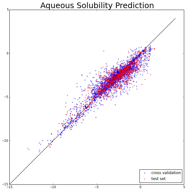
The aqueous solubility prediction. The X-axis represents experimental values and the Y-axis represents predicted values.
1 2 3 4 5 6 7 8 9 10 11 12 13 14 15 16 17 18 19 20 21 22 23 24 25 26 27 28 29 30 31 32 33 34 35 36 37 38 39 40 41 42 43 44 45 46 47 48 49 50 51 52 53 54 55 56 57 58 59 60 61 | from PyBioMed import Pymolecule
import pandas as pd
import numpy as np
from sklearn import cross_validation
from sklearn.ensemble import RandomForestRegressor
from matplotlib import pyplot as plt
from sklearn.cross_validation import train_test_split
from sklearn import metrics
#==============================================================================
# loading the data
#==============================================================================
#change the path to your own path
solubility_set = pd.read_excel('./example/solubility/Solubility-total.xlsx',sheetname = 0)
smis = solubility_set['SMI']
logS = solubility_set['logS']
#==============================================================================
# #calculating molecular descriptors
#==============================================================================
def calculate_des(smi):
des = {}
drugclass=Pymolecule.PyMolecule()
drugclass.ReadMolFromSmile(smi)
des.update(drugclass.GetEstate())
des.update(drugclass.GetMOE())
return pd.DataFrame({smi:(des)}).T
solubility_set_des = pd.concat(map(calculate_des,list(smis)))
solubility_set_des = np.array(solubility_set_des)
logS = np.array(logS)
#==============================================================================
# building the model and predict
#==============================================================================
train_set_des, test_set_des, train_logS, test_logS = train_test_split(solubility_set_des,
logS, test_size = 0.33, random_state = 42)
kf = cross_validation.KFold(train_set_des.shape[0], n_folds=10, random_state=0)
clf = RandomForestRegressor(n_estimators=500, max_features='auto', n_jobs = -1)
CV_pred_logS = []
VALIDATION_index = []
for train_index, validation_index in kf:
VALIDATION_index = VALIDATION_index + list(validation_index)
clf.fit(train_set_des[train_index ,:],train_logS[train_index])
pred_logS = clf.predict(train_set_des[validation_index,:])
CV_pred_logS = CV_pred_logS + list(pred_logS)
CV_true_logS = train_logS[VALIDATION_index]
r2_CV = metrics.r2_score(CV_true_logS, CV_pred_logS)
clf.fit(train_set_des,train_logS)
pred_logS_test = clf.predict(test_set_des)
r2_test = metrics.r2_score(test_logS, pred_logS_test)
#==============================================================================
# plotting the figure
#==============================================================================
plt.figure(figsize = (10,10))
plt.plot(range(-15,5),range(-15,5),'black')
plt.plot(CV_true_logS,CV_pred_logS,'b.',label = 'cross validation', alpha = 0.5 )
plt.plot(test_logS,pred_logS_test,'r.',label = 'test set',alpha = 0.5)
plt.title('Aqueous Solubility Prediction',{'fontsize':25})
plt.legend(loc="lower right",numpoints=1)
plt.plot()
|
>>> print 'CV_R^2:',r2_cv,'Test_R^2:',r2_test
CV_R^2: 0.86 Test_R^2: 0.84
Application 3 Prediction of drug–target interaction from the integration of chemical and protein spaces
Drug-target interactions (DTIs) are central to current drug discovery processes and public health fields. The rapidly increasing amount of publicly available data in biology and chemistry enables researchers to revisit drug-target interaction problems by systematic integration and analysis of heterogeneous data. To identify the interactions between drugs and targets is of important in drug discovery today. Interaction with ligands can modulate the function of many targets in the processes of signal transport, catalytic reaction and so on. With the enrichment of data repository, automatically prediction of target-protein interactions is an alternative method to facilitate drug discovery. Our previous work (Cao et al, 2014) proved that the calculated features perform well in the prediction of chemical-protein interaction. The benchmark data set for building the drug-target interaction predictor was taken from (Yamanishi, Araki et al. 2008). The dataset contains 6888 samples, among them 2922 drug-protein pairs have interactions which are defined as positive dataset and 3966 drug-protein pairs do not have interactions which are defined as negative dataset. To represent each drug-protein pairs, 150 CATS molecular fingerprints and 147 CTD composition, transition and distribution features of protein, a total number of 297 features were used. The random forest (RF) classifier was employed to build model.
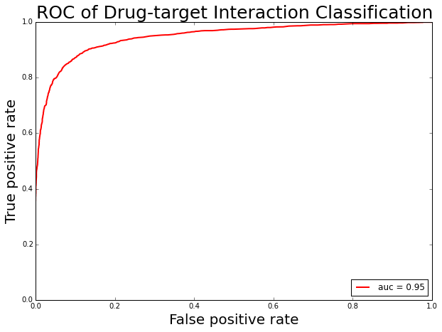
The receiver operating characteristic curve of drug-target interaction classification.
1 2 3 4 5 6 7 8 9 10 11 12 13 14 15 16 17 18 19 20 21 22 23 24 25 26 27 28 29 30 31 32 33 34 35 36 37 38 39 40 41 42 43 44 45 46 47 48 49 50 51 52 53 54 55 56 57 58 59 60 61 62 63 64 65 66 67 68 69 70 71 72 73 74 75 76 77 78 79 80 81 82 83 84 85 86 87 88 | from PyBioMed import Pymolecule
from PyBioMed import Pyprotein
import pandas as pd
import numpy as np
from sklearn.ensemble import RandomForestClassifier as RF
from sklearn import cross_validation
from sklearn import metrics
from matplotlib import pyplot as plt
#==============================================================================
# loading the data
#==============================================================================
path = 'input PyBioMed path in your computer' #input the real path in your own path
smis = pd.read_excel(path + 'example/dpi/DPI_SMIs.xlsx')
smis.index = smis['Drug']
protein_seq = pd.read_table(path + 'example/dpi/hsa_seqs_all.tsv', sep = '\t')
protein_seq.index = protein_seq['Protein']
positive_pairs = pd.read_excel(path + 'example/dpi/Enzyme.xls')
positive_pairs = zip(list(positive_pairs['Protein']), list(positive_pairs['Drug']))
negative_pairs = pd.read_excel(path + 'example/dpi/Enzymedecoy.xls')
negative_pairs = zip(list(negative_pairs['Protein']), list(negative_pairs['Drug']))
#==============================================================================
# calculating descriptors
#==============================================================================
def calculate_pair_des(smi, seq):
pair_des = {}
drugclass = Pymolecule.PyMolecule()
drugclass.ReadMolFromSmile(smi)
pair_des.update(drugclass.GetCATS2D())
proclass = Pyprotein.PyProtein(seq)
pair_des.update(proclass.GetCTD())
return pair_des
positive_pairs_des = {}
for n, positive_pair in enumerate(positive_pairs):
try:
pair_des = calculate_pair_des(smis.ix[positive_pair[1]][1],protein_seq.ix[positive_pair[0]][1])
positive_pairs_des[n] = pair_des
except:
continue
negative_pairs_des = {}
for n, negative_pair in enumerate(negative_pairs):
try:
pair_des = calculate_pair_des(smis.ix[negative_pair[1]][1],protein_seq.ix[negative_pair[0]][1])
negative_pairs_des[n] = pair_des
except:
continue
#==============================================================================
# cross-validation
#==============================================================================
x = np.array(pd.concat([pd.DataFrame(positive_pairs_des).T, pd.DataFrame(negative_pairs_des).T],
join_axes=[pd.DataFrame(positive_pairs_des).T.columns],axis = 0, ignore_index=True))
positive_count, negative_count = len(positive_pairs_des), len(negative_pairs_des)
y = np.array([1]*positive_count+ [0]*negative_count)
# ROC curve of CV
kf = cross_validation.KFold(x.shape[0], n_folds=10, shuffle=True,random_state=5)
clf = RF(n_estimators=500, max_features='sqrt', n_jobs=-1, oob_score=True)
CV_pred_prob = []
CV_pred_label=[]
VALIDATION_index = []
for train_index, validation_index in kf:
VALIDATION_index = VALIDATION_index + list(validation_index)
clf.fit(x[train_index ,:],y[train_index])
pred_prob = clf.predict_proba(x[validation_index,:])
pred_label = clf.predict(x[validation_index,:])
CV_pred_prob = CV_pred_prob + list(pred_prob[:,1])
CV_pred_label = CV_pred_label + list(pred_label)
fpr_cv, tpr_cv, thresholds_cv = metrics.roc_curve(y[VALIDATION_index], CV_pred_prob)
y_true = y[VALIDATION_index]
AUC_score = metrics.roc_auc_score(y[VALIDATION_index], CV_pred_prob)
TPR = metrics.recall_score(y_true, CV_pred_label)
ACC = metrics.accuracy_score(y_true, CV_pred_label)
SPE = (float(positive_count)/float(negative_count)+1.0)*ACC-TPR*float(positive_count)/float(negative_count)
matthews_corrcoef = metrics.matthews_corrcoef(y_true, CV_pred_label)
f1_score = metrics.f1_score(y_true, CV_pred_label)
#==============================================================================
# plotting the figure
#==============================================================================
plt.figure(figsize = (10,7))
plt.plot(fpr_cv, tpr_cv, 'r', label='auc = %0.2f'% AUC_score, lw=2)
plt.xlabel('False positive rate',{'fontsize':20});
plt.ylabel('True positive rate',{'fontsize':20});
plt.title('ROC of Drug-target Interaction Classification',{'fontsize':25})
plt.legend(loc="lower right",numpoints=15)
plt.show()
|
>>> print 'sensitivity:',TPR, 'specificity:', SPE, 'accuracy:', ACC, 'AUC:', AUC_score, 'MCC:', matthews_corrcoef, 'F1:', f1_score
sensitivity: 0.84 specificity: 0.93 accuracy: 0.89 AUC: 0.95 MCC: 0.78 F1: 0.87
Application 4 Prediction of protein subcellular location
To identify the functions of proteins in organism is one of the fundamental goals in cell biology and proteomics. The function of a protein in organism is closely linked to its location in a cell. Determination of protein subcellular location (PSL) by experimental methods is expensive and time-consuming. With the enrichment of data repository, automatically prediction of PSL is an alternative method to facilitate the determination of PSL. To build a PSL prediction model, we use PyProtein in PyBioMed to calculate protein features and then the random forest (RF) method was applied to build PSL classification model. The benchmark data set for building the protein subcellular location predictor was taken from (Jia, Qian et al. 2007). The dataset contains 2568 samples, among them 849 proteins were located at Cytoplasm which is defined as positive dataset and 1619 proteins were located at Nucleus which is defined as negative dataset. For each protein, 20 amino acid composition (AAC), 147 CTD composition, transition and distribution and 30 pseudo amino acid composition (PAAC), a total number of 197 features were calculate through the PyBioMed tool.
To build the classification model, the CSV file containing the calculated descriptors was then converted to sample matrix (x_train) and a sample label vector (y_train) is also provided. Then, the python script randomforests.py based on sklearn package was employed to build the classification model (the number of trees is 500, the maximum number of features in each tree is square root of the number of features). The performance of this model was evaluated by using 10-fold cross-validation. The AUC score, accuracy, sensitivity and specificity are 0.90, 0.85, 0.94 and 0.69 respectively

The receiver operating characteristic curve of protein subcellular location classification.
1 2 3 4 5 6 7 8 9 10 11 12 13 14 15 16 17 18 19 20 21 22 23 24 25 26 27 28 29 30 31 32 33 34 35 36 37 38 39 40 41 42 43 44 45 46 47 48 49 50 51 52 53 54 55 56 57 58 59 60 61 62 63 64 65 | import pandas as pd
from PyBioMed.PyProtein.CTD import CalculateCTD
import numpy as np
from sklearn.ensemble import RandomForestClassifier as RF
from sklearn import cross_validation
from sklearn import metrics
from matplotlib import pyplot as plt
#==============================================================================
# loading the data
#==============================================================================
path = 'input PyBioMed path in your computer' #input the PyBioMed path in your own computer
f = open(path + 'example/subcell/Cytoplasm_seq.txt','r')
cytoplasm = [line.replace('\n','') for line in f.readlines() if line != '\n']
f.close()
f = open(path + 'example/subcell/Nuclear_seq.txt','r')
nuclear = [line.replace('\n','') for line in f.readlines() if line != '\n']
f.close()
#==============================================================================
# calculating the descriptors
#==============================================================================
cytoplasm_des = dict(zip(range(len(cytoplasm)),map(CalculateCTD,cytoplasm)))
nuclear_des = dict(zip(range(len(nuclear)),map(CalculateCTD,nuclear)))
cytoplasm_des_df = pd.DataFrame(cytoplasm_des).T
nuclear_des_df = pd.DataFrame(nuclear_des).T
#==============================================================================
# cross-validation
#==============================================================================
x = np.array(pd.concat([cytoplasm_des_df, nuclear_des_df]))
positive_count, negative_count = len(cytoplasm_des), len(nuclear_des)
y = np.array([1]*positive_count+ [0]*negative_count)
kf = cross_validation.KFold(x.shape[0], n_folds=10, shuffle = True, random_state=5)
clf = RF(n_estimators=500, max_features='sqrt', n_jobs=-1, oob_score=True)
CV_pred_prob = []
CV_pred_label=[]
VALIDATION_index = []
kf = cross_validation.KFold(x.shape[0], n_folds=10, shuffle=True,random_state=5)
clf = RF(n_estimators=500, max_features='sqrt', n_jobs=-1, oob_score=True)
CV_pred_prob = []
CV_pred_label=[]
VALIDATION_index = []
for train_index, validation_index in kf:
VALIDATION_index = VALIDATION_index + list(validation_index)
clf.fit(x[train_index ,:],y[train_index])
pred_prob = clf.predict_proba(x[validation_index,:])
pred_label = clf.predict(x[validation_index,:])
CV_pred_prob = CV_pred_prob + list(pred_prob[:,1])
CV_pred_label = CV_pred_label + list(pred_label)
fpr_cv, tpr_cv, thresholds_cv = metrics.roc_curve(y[VALIDATION_index], CV_pred_prob)
y_true = y[VALIDATION_index]
AUC_score = metrics.roc_auc_score(y[VALIDATION_index], CV_pred_prob)
TPR = metrics.recall_score(y_true, CV_pred_label)
ACC = metrics.accuracy_score(y_true, CV_pred_label)
SPE = (float(positive_count)/float(negative_count)+1.0)*ACC-TPR*float(positive_count)/float(negative_count)
matthews_corrcoef = metrics.matthews_corrcoef(y_true, CV_pred_label)
f1_score = metrics.f1_score(y_true, CV_pred_label)
#==============================================================================
# plotting the figure
#==============================================================================
plt.figure(figsize = (10,7))
plt.plot(fpr_cv, tpr_cv, 'r', label='auc = %0.2f'% AUC_score, lw=2)
plt.xlabel('False positive rate',{'fontsize':20});
plt.ylabel('True positive rate',{'fontsize':20});
plt.title('ROC of protein subcellular location Classification',{'fontsize':25})
plt.legend(loc="lower right",numpoints=15)
plt.show()
|
>>> print 'sensitivity:',TPR, 'specificity:', SPE, 'accuracy:', ACC, 'AUC:', AUC_score, 'MACCS:', matthews_corrcoef, 'F1:', f1_score
sensitivity: 0.67 specificity: 0.92 accuracy: 0.84 AUC: 0.89 MACCS: 0.62 F1: 0.74
Application 5 Predicting nucleosome positioning in genomes with dinucleotide-based auto covariance
Nucleosome positioning participates in many cellular activities and plays significant roles in regulating cellular processes (Guo, et al., 2014). Computational methods that can predict nucleosome positioning based on the DNA sequences is highly desired. Here, a computational predictor was constructed by using dinucleotide-based auto covariance and SVMs, and its performance was evaluated by 10-fold cross-validation. The benchmark data set for the H. sapiens was taken from (Schones, et al., 2008). Since the H. sapiens genome and its nucleosome map contain a huge amount of data, according to Liu’s strategy (Liu, et al., 2011) the nucleosome-forming sequence samples (positive data) and the linkers or nucleosome-inhibiting sequence samples (negative data) were extracted from chromosome (Guo, et al., 2014). A file named “H_sapiens_pos.fasta” containing 2,273 nucleosome-forming DNA segments is used as the positive dataset, and a file named “H_sapiens_neg.fasta” containing 2,300 nucleosome-inhibiting DNA segments is used as the negative dataset.

The receiver operating characteristic curve of nucleosome positioning in genomes classification.
1 2 3 4 5 6 7 8 9 10 11 12 13 14 15 16 17 18 19 20 21 22 23 24 25 26 27 28 29 30 31 32 33 34 35 36 37 38 39 40 41 42 43 44 45 46 47 48 49 50 51 52 53 54 55 56 57 58 59 60 61 62 63 64 65 66 67 68 | import pandas as pd
from PyBioMed import Pydna
from PyBioMed.PyGetMol import GetDNA
import numpy as np
from sklearn.ensemble import RandomForestClassifier as RF
from sklearn import cross_validation
from sklearn import metrics
from matplotlib import pyplot as plt
#==============================================================================
# loading data
#==============================================================================
path = 'PyBioMed package real path in your computer' # input the real path in your own computer
seqs_pos = GetDNA.ReadFasta(open(path + '/example/dna/H_sapiens_pos.fasta'))
seqs_neg = GetDNA.ReadFasta(open(path + '/example/dna/H_sapiens_neg.fasta'))
#==============================================================================
# calculating descriptors
#==============================================================================
def calculate_des(seq):
des = []
dnaclass = Pydna.PyDNA(seq)
des.extend(dnaclass.GetDAC(all_property=True).values())
des.extend(dnaclass.GetPseDNC(all_property=True,lamada=2, w=0.05).values())
des.extend(dnaclass.GetPseKNC(all_property=True,lamada=2, w=0.05).values())
des.extend(dnaclass.GetSCPseDNC(all_property=True).values())
return des
pos_des = []
for seq_pos in seqs_pos:
pos_des.append(calculate_des(seq_pos))
neg_des = []
for seq_neg in seqs_neg:
neg_des.append(calculate_des(seq_neg))
#==============================================================================
# cross validation
#==============================================================================
x = np.array(pos_des+neg_des)
positive_count, negative_count = len(pos_des), len(neg_des)
y = np.array([1]*positive_count+ [0]*negative_count)
kf = cross_validation.KFold(x.shape[0], n_folds=10, random_state=0)
clf = RF(n_estimators=500, max_features='sqrt', n_jobs=-1, oob_score=True)
CV_pred_prob = []
CV_pred_label=[]
VALIDATION_index = []
for train_index, validation_index in kf:
VALIDATION_index = VALIDATION_index + list(validation_index)
clf.fit(x[train_index ,:],y[train_index])
pred_prob = clf.predict_proba(x[validation_index,:])
pred_label = clf.predict(x[validation_index,:])
CV_pred_prob = CV_pred_prob + list(pred_prob[:,1])
CV_pred_label = CV_pred_label + list(pred_label)
fpr_cv, tpr_cv, thresholds_cv = metrics.roc_curve(y[VALIDATION_index], CV_pred_prob)
# Calculate auc score of cv
y_true = y[VALIDATION_index]
AUC_score = metrics.roc_auc_score(y[VALIDATION_index], CV_pred_prob)
TPR = metrics.recall_score(y_true, CV_pred_label)
ACC = metrics.accuracy_score(y_true, CV_pred_label)
SPE = (float(positive_count)/float(negative_count)+1.0)*ACC-TPR*float(positive_count)/float(negative_count)
matthews_corrcoef = metrics.matthews_corrcoef(y_true, CV_pred_label)
f1_score = metrics.f1_score(y_true, CV_pred_label)
#==============================================================================
# plotting the figure
#==============================================================================
plt.figure(figsize = (10,7))
plt.plot(fpr_cv, tpr_cv, 'r', label='auc = %0.2f'% AUC_score, lw=2)
plt.xlabel('False positive rate',{'fontsize':20});
plt.ylabel('True positive rate',{'fontsize':20});
plt.title('ROC of Nucleosome Positioning in Genomes Classification',{'fontsize':25})
plt.legend(loc="lower right",numpoints=15)
plt.show()
|
>>> print 'sensitivity:',TPR, 'specificity:', SPE, 'accuracy:', ACC, 'AUC:', AUC_score, 'MACCS:', matthews_corrcoef, 'F1:', f1_score
sensitivity: 0.82 specificity: 0.80 accuracy: 0.81 AUC: 0.88 MACCS: 0.62 F1: 0.81